Distortion
Hello, dear readers! In this article we will speak about distortion algorithms, and about thousands other useful things, for example decibels, Bezier curves of arbitrary orders and the Newton method.
Note: everywhere below I will refer to the term "sample" as a number, not as a whole sound!
We will start from the decibels measuring, because this is important in audio applications.
Let's start!
Decibels Measuring
1. Definition
2. Decibels for sample level measuring
3. Decibels for gain (amplification coefficient) measuring
4. Implementation
1. Definition
Let's chat about some units of measurement. What do you think when you hear the word "unit"? For example, ampere. It is a so-called absolute, objective unit. If I remember right from school physics, it measures how much charge goes through the circuitry in the amount of time equal to 1 second. As the second also has a strict definition and can be computed, if my memory serves me well, from some astronomic constants, then we will understand that ampere is a self-sufficient unit. In fact, we don't have to know anything to understand ampere correctly, i.e. when somebody says that the amperage in a circuitry is 2 ampere, everyone will understand him correctly (if they aren't fools, of course). 2 ampere are 2 ampere - not more, not less.
But now let's come to decibels. Here this rule isn't right: 2 db aren't 2 db, in general case! How can this be possible?
The answer is short: because decibel isn't a common unit, and you often won't even find it in some reference books. It has a absolutely different structure, another meaning than all standard values. They measure absolute values, decibels - relative.
Now it's time to give the definition.
DEFINITION: Decibel is a value which measures the correlation between two values, we get it from the following formula:
        I = 10 * log     I1
                    10  ----
                         I2
where I1 and I2 are two values which we measure. So, two values are "merged" into one value, in decibels.
In practice we want to get the power of sound, not its current strength or voltage. In electronic devices it might be hard to measure the power concretely. So, people measure its current strength and then use the formula P = R * I^2.
So, power relations in decibels become equal to
    10 * log     R * I1^2   10 * log   (I1/I2)^2 = 20 * log   (I1/I2)
P=          10   -------- =         10                     10
                 R * I2^2
- The logarithm of a^x is equal to x*log(a).
So, decibel values have a logarithmic structure.
Where are they used? Everywhere in physics. Acoustics, electricity, electronics etc. Some people think that decibel is used only in acoustics for "volume" measurement. They are wrong. Decibel is also used in voltage comparisons, for example. And, if to dip into history, we will discover that decibel was invented in Bell's (inventor of the telephone) company, at the beginning of the XXth century, for convenient work with gains of telephone amplifiers. They had hard calculations if two amplifiers were connected in the serial way, then their output gain is calculated by multiplication of their individual gains. They introduced this logarithmic scale, and, if you remember school, log(A*B) = log(A) + log (B) and log(A/B) = log(A) - log(B). So, when they needed to multiply gains, they just added their values in decibels, and then found the antilogarithm from this value (by huge books with huge tables - I have one of them - reliquiae :).
So, you see - to measure something in decibels we should have "something" for comparison, for I2. When you read that a signal is -6 db this means absolutely nothing. Only when you know what exactly was taken for I2 (or 0 db) in the formula of decibels, you can judge. So, decibel isn't a self-sufficient unit of measurement.
In acoustics (not in digital sound) for sound measuring one constant is used (I don't know its exact value, look in references for this, if you're interested), it is the minimal power which sound should have in order to be heard.
Finally, if you wonder why you should use decibel: Maybe you want to do everything in plain sample values, why to use decibels instead - after all, they lead to an undesired amount of calculations? Then I have one question to you - have you ever seen normal sound programs in which the sample values aren't in decibel (except old trackers - they aren't normal programs)? I haven't ever seen this, if you've seen any of this sort then show them to me. So, there should be an objective reason why these big companies use decibels, and they are professionals, so they must have reasons.
And the main reason comes from the physics of the ear. It has been proven that our ears perceive loudness not in a linear, but in a logarithmical way. So, understand why decibel is useful? When you apply gain 2 to your music, i.e. multiply every element with 2, you won't get music which sounds twice as loud. Only if you apply gain 2 db, you will get such a difference in loudness. And 2 db is "bigger" than 2. But whether "bigger" it or "smaller" we will know only from the following two sections.
2. Decibels for sample level measuring
Now let's come closer to digital sound. As we know, we should take some value for comparison in db calculating. But which? If you are good at mathematics, you can go to the sample editor and there examine the db ruler. You will notice that it goes from -infinity to 0 db. We know that db are logarithmic values, in fact. Where are logarithms negative? From 0 to 1. So, it's obvious that in the main formula of decibels we should have such relation, which becomes 1 at the maximal sample level, so, the logarithm of 1 will be equal to 0. What to take for I2 or 0 db? It's simple - you should take for the zero level the maximal positive constant which is possible in your current digital audio representation.
For 16-bit signed audio this constant is 32767 - it's the maximal possible positive constant for this data type. For 8-bit signed audio - 255. For 32 bit - well, calculate yourself, 2^32 - 1.
When we have chosen an appropriate reference value (let's write it as I0), we can compute decibels.
For example, we look at our array with sample data and see that in the current place stands value 16384 (plain sample value, not in db). Let's write it as I. We should get its decibels representation. Use the formula:
P = 20 * log    I
            10 ---
                I0
In this case this is equal to I = 20*lg(16384/32767) = -6.0 db
Ah, yes, one thing - it is commonly accepted to write decibels with a precision of one sign after the fractal point, so don't bother yourself with precise calculations.
If you haven't understood the matter from my words, then read this piece from Sound Forge User's Manual:
"In Sound Forge, most measurements are given in decibels. For example, if you want to double the amplitude of a sound, you apply a 6 dB gain. A sample value of 32,767 (maximum positive sample value for 16-bit sound) can be referred to as having a value of 0 dB. Likewise, a sample value of 16,384 can be referred to having a value of -6 dB."
Now another problem - how to compute the normal sample value if we know its value in decibels?
Another simple school task - we have the value P. So,
log    I     P
   10 --- = ---
       I0    20
Now you should recall the definition of logarithm. We know (at least, should know) that
log n = k
   m
is identical (by definition) with m^k = n.
So, the task is simple:
10^(P/20) = I/I0

Now I = I0 * 10^(P/20) = I0 * 10^(P/20)
About faster implementation of this calculations you may read in one of the following chapters.
Now another useful note: when you need to calculate a value in decibels from a negative sample value, you should use its absolute value, because logarithms aren't defined for negative numbers.
3. Decibels for gain measuring.
Now recall your favourite sound editing program. Recall, when you apply some transformations, you should specify their amount, i.e. how much the processed signal will be mixed with the original one. In all programs these values are specified in decibels. But it's obvious that now we shouldn't use the same formula as for sample levels. Instead of this we measure the relative amount of one parameter, taken before and after the transformation, so in the decibels formula this parameter goes away, allowing you to calculate decibels using only one number.
Example: Let's say we should amplify sound with the gain 6 db.
For this our program should know the "value" of 6 db, because we can't multiply our samples on 6 db, right? We need the normal gain value. So, let's agree that before the transformation our signal had power P, after it - n*P, where n is the desired gain. The user has specified the amount of gain in db, let's write it as A. Let's write the formula:
A = 20 * log   n*P
            10 --- = 20 * log   n
                P            10
We see that P has gone away, we don't need it.
Now let's find n from this.
log   n = A/20
   10
so, n = 10^(A/20).
Example: The user has specified an amount of gain equal to 13 db. What is the exact coefficient of multiplication for our digital amplifier?
Solution: Use the above formula. Here A = 13 db. We should find n. Let's do it.
n = 10^(13/20) = 10^0.65 = 4.46
Our original signal should be multiplied by 4.46 to become amplified by 13 db.
4. Implementation
First, about the calculation of logarithms. If you write in your program something like
level_in_db = 20 * log(A/32767),
then, of course, you will get an incorrect answer. Look: our formula for calculation of decibels looks like:
20 log   (I/I0)
      10
Here we should use decimal logarithms, while "log" stands for natural logarithms in C and Pascal, with base e, not 10. For decimal logarithms in C there's a function log10, which we need to use (both of these functions, log and log10, are defined in the mathematical module, so you should include the header file "math.h" in your program). In Pascal and other languages where there's no log10 function you should write it for yourself - this is easy:
We know:
  log    c  = log  c
      b          d
              ------
              log  b
                 d
So,
  log     c = ln c
      10      -----
              ln 10
So, now you can use the standard function "ln" (or any other name that is used in the particular language for this).
I suppose there's no need to say that you should compute the constant (1/ln(10)) only once, and then calculate your values by multiplying ln on this, not by dividing?
For reverse calculations, for the formula 10^(A/20) we should use the notation pow10(A/20) in C. For other languages we should use the regular formula for the calculation of an arbitrary power of a number. Here's how it is derived:
1) axiom one: e^(ln x) = x (e^x is written like exp(x))
2) axiom two: ln(a^b) = b*ln(a)
3)
             b
         ln a       b    b*ln(a)
        e        = a  = e        = exp(b*ln(a))
So, a^b = exp(b*ln(a))
Of course, all those calculations take a lot of time, if to take in account the fact that we are dealing with samples, with high discretization rates, and they should be applied to every single sample. Of course, in realtime applications something else should be introduced.
Tables, of course.
The simplest method that flows on mind is to sacrifice 64*n kb (n is size of your favourite data type) of memory for a table for one-side calculation (either sample->decibels, or decibels->sample). And then our process could be described like this:
calculate decibels from sample value A
{
        Look in table (A);
        if (Present) then return table[A];
        else return Calculate decibels(A);
}
So, we won't need to calculate the same values twice (thrice, ...), only once. Something like a cache.
However, this situation works only for 16-bit audio - our table is 64k * sizeof(type). 64k is 2^16. If we use 32-bit samples, we should introduce 2^32 * sizeof(type) table, and, errm, this is far more than the amount of memory available for 32-bit processors.
So, of course, the implementation of this look-up tables for 32-bit data is impossible now (and won't be used even when the amount of memory will exceed all those numbers).
We have to find another way of looking up. And, of course, it exists. Its name is: Hash Tables.
I plan to write an article about them for the next Hugi, so you have to wait if you don't know them.
Basically, they are non-sorted arrays, where the time of search approaches O(1) - in the best case.
Now we could move further, to our main topic - distortion.
Parametric Distortion
This is one of the most basic DSP effects, in fact. Why is it called parametric? Because you just have four variables for its control: Dry Level, Wet Level, Threshold and Clamping Level. Let's discover the inner working of such a distorter, and these parameters will become obvious,
First, this effect is a single-sample effect, at every moment we work only with one sample value, not with a group of them. Let the distorter get its data from array input. It takes the current sample, and begins to analyze it. If its level (sample value in db) is greater than or equal to a specified constant (Threshold Level), the distorter yields a sample whose value is Clamping Level. Then the "distorted" output - this sample - is scaled to Wet (Distorted) Level - in db, of course. After this procedure we add the original sample value to this "distorted" value, where the original sample value is scaled according to the Dry Level parameter.
Here's several examples for understanding:
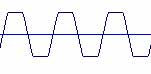
Here the following parameters are used:
Dry level = -inf db (means no original signal at all)
Wet level = 0 db (means no additional amplification)
Threshold level = -19 db
Clamping level = -19 db
You see, here, just when the signal exceeds -19 db, it is "truncated" to these -19 db.
So, our original sine wave is cut now.
Little note: Clamping level = Threshold level is quite a good preset almost in any case.
Also we can get interesting results, for example, how to make a sine wave form more "fat"?
Simply raise up the dry level from -inf to a higher amount of decibels. The original wave, when summed with distorted, will produce this "fatness". Example:
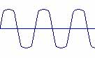
Here all parameters are the same as in the first picture except dry level, which is -16 db now.
So, I suppose, everything is easy, and it's very easy to code it, like:
void distortion(short threshold, short level, float dry, float distorted)
{
        for (i=0; i<=length_of_sound-1; ++i)
        {
                if (abs(output[i])>threshold)
                   output[i]=dry*output[i]+sign(output[i])*distorted*level;
                else output[i]=output[i]*(dry + distorted);
        }
}
The parameters in this procedure call are already plain values, I mean converted from decibels.
Of course, this isn't optimal, and should be rewritten in assembly for cool speed. This is your problem.
This type of distortion, parametric distortion, is used in many "simple" programs, and even in Sound Forge. In fact, it does its job good, it's fast and small.
But sometimes such parameters become inconvenient for specific tasks, or such a little amount of control (4 variables) is too little.
Here we can forget this parametric scheme and use another approach, which is more sophisticated, but also more time-consuming.
So,
Functional distortion
Sorry, I've "composed" this term for myself, because our control will be one function instead of four control variables, and maybe in our sources it is called another way.
This type of distortion is used in Cool Edit Pro, and if you used it, you will understand me clearly.
Let's look what Cool Edit Pro has to offer:
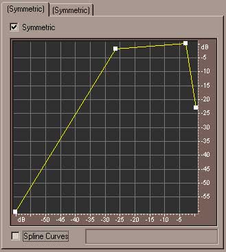
As you see, there's no other controls except one graph. What does it show us?
Imagine two axes - x and y. Then remember that towards the x axis we have sample values in the input signal, and towards the y axis we have sample values in the output signal.
It means the following: when the program "sees" that the current sample has the value, let's say, -12db, it "looks" at this graph, finds this value at the x axis and then calculates what value our function (yellow curve) has in this point. And then it changes the original sample value by this founded sample value.
You see, this is a very general and convenient approach, because to made Cool Edit Pro compressor, for example, you need to add only volume-measurer to this approach.
Obvious, that all those parametric schemes we discussed earlier could be presented on this graph, but not any curve in a graph could be presented using the parametric approach, of course.
That is why we use this model - to generalize and to ravel your program (and to make it slooow, like Cool Edit :)).
So, how to present old parametric schemes in this approach? All of them have the same form, something like this:
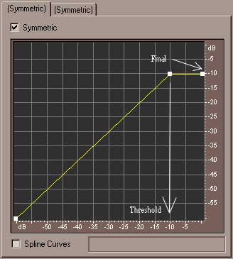
In this picture the threshold level is at -10 db, and clamping level is also at -10 db.
You see, below -10 db our signal remains the same, but when it starts to exceed -10 db, distorter changes any greater value to -10 db.
But, err, all of this you can read in the corresponding user manuals. Our main part:
Implementation
So, the algorithm is obvious: get input value, compute the distortion function from this parameter, store this "distorted" sample in the output array.
The hardest part here is how to maintain and calculate this function.
We are able to specify any amount of control points on this graph, and, generally, it can approximate any curve. So, we need to store these points in the memory (genious!).
Now we have two ways: either store them in an array, or in the form of dynamic lists. We should use the first type. Why? Because in the time of calculation of our function we will need to find the appropriate point in this array, and in linked lists we can use only one algorithm of search - sequential search, when you have to start every time from the begining of the lists and search until it appear. But in arrays we already can use a more efficient algorithm - dichotomic search. But later about it.
So, our approach: the control points on the graph are stored in the array, let's call it "points".
Now we should imagine the next step: we get a value, we should compute our function from it. The graph consists only of straight lines. So, we have all the basic sources. We know that a line is strictly defined by two control points. And the idea is: to find where, between what control points our point lies. In operations of addition and deletion of control points you should treat your points array as sorted and preserve this, i.e. when the user adds a control point, you should place it in the appropriate position in the array (according to the x coordinate).
As I have already said, we chose an array because of its ability to perform dichotomic search in it (for this type of search, the array should be sorted - that is why I told you to preserve this while adding and deleting control points). So, now we should find two points in our array, between which our desired point lies, and then we will be able to calculate the equation of the line between these two points, and then find the desired y for the specified x.
In dichotomic search, if you don't know, we choose the central element in the array and compare it with the number which should be found. If our array is sorted in ascending order, and if we've found that our value is less than the central value, we continue our search in left part of array. It is logical, for example consider the array 1, 2, 3, 4, 5, 6, 7, 8, 9, 10. We should find 3. The central element is 5. 3<5. And, because this array is sorted, we see that it simply should be to the left of the central element, if it is present in the array, of course.
So, the idea is obvious. Of course, in our task we shouldn't search exactly the desired value, because we won't always find it, we should search a point that is smaller than our number and the next point being bigger than our number. I suppose, it is sufficient for understanding?
One problem has been solved. Now another one. We've found two points, between which lies our point. We should construct the equation of the line between these points, and then, knowing only x on this line, get y for this x.
We have two points, P0 and P1. The equation of the line which goes through these points has the following form:
P = P0 + (P1-P0)*t
Note that P, P0, P1 are vectors, not numbers, it means that by this equation we instantly get a point on the line. This is a so-called parametric equation - it depends only on t, and if to get t from 0 to 1, we will get this line P0P1.
So, if we suppose that P has the coordinates x and y, P0 - (x0,y0), P1 - (x1,y1), this equation could be written as
{ x = x0 + (x1-x0)*t
{ y = y0 + (y1-y0)*t
We know this x (this is the value from the input array - current sample value), we also know those x0, y0, x1, y1. We should find y.
From the first equation:
t = (x-x0)
    -------
    (x1-x0)
Place it in the second equation:
y = y0 + (y1-y0)*(x-x0)
         --------------
            (x1-x0)
That's all - the problem is solved. Only note one useful thing, look at the fraction:
(y1-y0)
 -------
(x1-x0)
You see, it doesn't depend on x, it is constant; and what should we do with constants?
Store them, of course. These fractions could (and should) be placed into our array with points, i.e. we should include this number in our structure of point:
struct point
{
        int x,y;
        float k;
}
And let's agree that in the point with number n we store this value for points Pn and Pn+1.
That's all, everything works faster than without this small but useful thing.
Of course this method is too slow to compute it in the real time. For 16-bit audio this should be computed only once, to calculate the look-up table.
Is this all? No, look at the dialog box of Cool Edit Pro. You will notice a small check box called "Spline Curves". By using this option you transform your graph to a Bezier curve of n-th order, where n is the number of control points minus 1. What a Bezier curve is and how to deal with it we will discover in the next chapter.
Spline Curves
Let's consider the parametric equation of the line one more time,
        {x = x0 + (x1-x0)*t
        {y = y0 + (y1-y0)*t
Let's write it in a form of
        {x = x0*(1-t) + x1*t
        {y = y0*(1-t) + y1*t
Now we can treat this equation like one where (1-t) and (t) are coefficients, and x0, y0, x1, y1 are control points.
What do control points do? They specify our line, they "say" that the line will go from (x0,y0) to (x1,y1). As we see, these parametric equations are equations of 1st order.
Next, one question arises: maybe there are some other forms of such polynoms, with higher orders and a higher amount of control points? Of course, they exist. But not all of them are useful. Here we will discuss only Bezier Curves of n-th order, because Cool Edit Pro uses exactly them.
These curves were introduced in 1970 by French engineer Bezier, who worked on the body of a new Renault car. He needed something more useful than simple lines, for example for the bonnet of the engine.
With such curves you have n control points (then the curve has order n-1). This curve has the following properties:
1) It always goes through the first and last control points. It doesn't go through any other control points (at least, in general case).
2) It goes in the direction specified by the control points, which means that our curve will bend on its way in trying to approach all control points.
3) It lies in the convex hull of the control points. It means that if we connect all control points sequentially by straight lines, our curve will lie in this polygon, it won't go beyond its edges.
Also another reason to use Bezier curves is their convenience for artists.
So, now we should discover the inner structure of the Bezier curves.
A Bezier curve is a parametric equation of n-th order with coefficients calculated by the Casteljau formula:
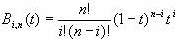
where n is the order of curve, i - the number of coefficients, t - the current value of the parameter.
What the hell does it mean? It means that our curve is represented by the following parametric equation:
x = B0*x0 + B1*x1 + ... + Bn*xn
y = B0*y0 + B1*y1 + ... + Bn*yn
where (x0,y0), (x1,y1), ..., (xn,yn) are the control points, B0, ..., Bn - coefficients, calculated from the above formula.
First step, let's find the coefficients for the curve of second order. The number of coefficients will be 3.
B0 =     2!
     -------- * (1-t)^(2-0)*t^0 = (1-t)^2
     0!(2-0)!

B1 =     2!
     -------- * (1-t)^(2-1)*t^1 = 2*t*(1-t)
     1!(2-1)!

B2 =     2!
     -------- * (1-t)^(2-2)*t^2 = t^2
     2!(2-2)!
Now the procedure of drawing of this curve will look like
void draw(control_points[], number_of_points)
{
float incr = 1.0/number_of_points;
float b0,b1,b2;
int x,y;

        for (float t=0; t<=1; t+=incr)
        {
                b0 = (1-t)*(1-t);
                b1 = 2*t*(1-t);
                b2 = t*t;

                x = b0*control_points[0].x + b1*control_points[1].x +
                        b2*control_points[2].x;
                y = b0*control_points[0].y + b1*control_points[1].y +
                        b2*control_points[2].y;

                putpixel(x,y);
        }
}
You see, to draw the whole Bezier curve we must iterate t from 0 to 1, with the desired step, the less the step, the higher the fidelity.
In this routine step (variable incr) is calculated by 1.0/number_of_points where number_of_points is the desired amount of points on our curve.
But, errm, this routine works only with second order curves, how to force it to draw curves of arbitrary order, we need this, because on that graph in Cool Edit Pro we can specify any number of control points?
How to calculate these coefficients Bi in real-time?
I submit the following approach made by me:
// ------------DEFINITIONS------------

struct POINT
  {
    double x,y;
  };

const order=10;     // order of curve

const N=1000;     // number of points on curve

typedef POINT CTRLPOINTS[order+1];      // array with control points

// ------------/DEFINITIONS-----------


double Power(double t, int n)       // routine of calculation of power, t^n
{
double rez=1;
const threshold = 10;               // when we should use straightforward calculation,
                                    // depends on concrete CPU
  if (n>treshold)
  {
    rez = exp(n*ln(t));             // straightforward calculation, when n is big
  } else
  {
    for (int i=1; i<=n; i++)        // iterative calculation
    {                               // good when in assembly and n is small
      rez *= t;
    }
  }

  return rez;
}


double CalculateCoefficient(int i, double t)    // heart of proc
{                                               // - calculation of Bi for t
static double rez;  // keyword static means that this variable will be statically
static int ifact;   // linked in this procedure, and when you enter here again and
static int temp;    // again, the content of this variable won't change, so you can
double coeff;       // conveniently use its previous value

  if (i==0)         // calculation of B0
  {
    rez = Power((1-t),order);   // B0 is always (1-t)^order

    coeff = 1;                  // coeff =     n!
                                //         ----------
                                //          i!*(n-i)!

    ifact = 1;                  // here we store i!, 0! = 1

    temp = order;               // temp =   n!
                                //        ------
                                //        (n-i)!
  } else
  {                             // next coefficients

    coeff = temp;               // recurrent calculation
    ifact *= i;                 // --//--
    coeff /= ifact;             // --//--
    temp *= (order - i);        // --//--
    rez /= (1-t);               // --//--
    rez *= t;                   // --//--
  }
  return rez*coeff;
}

POINT CalculateBezierPoint(double t, CTRLPOINTS points)  // calculate point for
{                                                        // specified t
POINT temp={0,0};
double coef;

  for(int i=0; i<=order; ++i)
  {
    coef = CalculateCoefficient(i,t);                   // calculate coeff. Bi

    temp.x += points[i].x * coef;       // x = b0*x0 + ... + bn*xn
    temp.y += points[i].y * coef;
  }
  return temp;
}

void DrawBezierCurve(int N, CTRLPOINTS points)  // main procedure
{
double incr = 1.0/N;                            // step

  for(double t=0; t <= 1; t+=incr)
  {
    POINT p = CalculateBezierPoint(t,points);   // calculate current point
                                                // for current t
    putpixel(p.x,p.y, GREEN);                   // draw points (or whatever you want)
  }
}
The heart of this program is the procedure CalculateCoefficient, it calculates the current Bi by using the previous Bi-1, using the technique of recurrent calculation.
Look, in each step we should multiply the previous coefficient by (1-t), and divide it by t.
And then multiply with the coefficient
    n!
---------
i!*(n-i)!
For calculation of this coefficient we use the following: n!/((n-i)!) is nothing else than regular factorial, but it goes not from 1 to n, but from n to 1. So, I recommend you just to put down on the sheet of paper each step of calculation of it, and everything will become obvious.
Note: This isn't pseudo-code but a working program, which works absolutely correctly (I believe). If anyone sees a mistake, please contact me.
So, one problem is solved, now we are able to calculate and draw points on the Bezier curve of n-th order. Very good for the beginning. But to actually implement a distorter based on the splines, we also need something else, to be able to calculate y for specified x on the Bezier curve, or how else could we compute the required output value for the distorter? Look, this is impossible in general case, because a Bezier curve neither depends on x nor on y but on t, it is a parametric curve.
So, the business becomes much more complicated. But let's kill this problem.
Newton Method
So, we have x(t) and y(t). Also we have specified x (input value). We should find t for this x, and then compute y(t) from this t. It can't be solved strictly, using formulas, because the polynom of n-th order has n roots, and for polynoms with degree >= 5 there are no formulae for finding their roots (theorem).
So, we should use approximation. Let's start with the Newton method, which converges very fast. But, of course, any thing has disadvantages and the Newton method isn't an exception.
Let's start. We have the equation
f(x) = k
We should find x from this equation.
Let's rewrite it in the form
f(x) - k = 0
Now, to find the roots of the equation, we should find the zeroes of the function (i.e. where this function, y = f(x) - k, is equal to zero).
Let's suppose that f(x) = x^2, k = 5. Watch the graph:
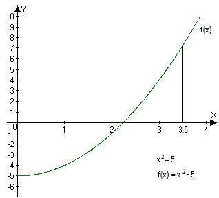
We have come to the first step in the Newton method:
1) To make the initial guess.
We should choose or "guess" (somehow) the initial x value, let's write it as x0.
In this example I chose x0 = 3.5 (here it is quite "doesn't matter").
Second step:
2) The next, closer approximation of x will be x1, which is computed as the
point where the tangent to f(x)-k in the point x0 is equal to zero.
Illustration:
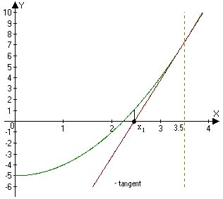
You see, just after a single iteration we've got a much closer answer from a random guess.
We can proceed with the same technique - now we should draw the tangent to f(x)-k in point x1, then the same-job-as-in-previous-iteration, and we get x2.
Now let's write this method in mathematical language, because now it is just pure words.
Let's find the formula for automatic calculation of xn from x(n-1).
So, we have x(n-1).
The equation of the tangent in this points to the function g(x) = f(x)-k:
y(x) = g(x(n-1)) + g'(x(n-1))*(x-x(n-1))
We should find such x where y(x) = 0.
0 = g(x(n-1)) + g'(x(n-1))*(x-x(n-1))

g'(x(n-1))*x(n-1) - g(x(n-1)) = g'(x(n-1))*x

x = x(n-1) - g(x(n-1))
             ----------
             g'(x(n-1))
So,
    xn = x(n-1) - g(x(n-1))
                  ----------   (1)
                  g'(x(n-1))
That's all with Newton method - everything is well formalised, we have a strict iteration formula for approximation.
Now we should apply this technique to our thing - the parametric Bezier curve.
Implementation
So, the algorithm is such:
1) We will find t for specified x by solving the equation x(t) - x = 0 using the Newton Method. After this we will calculate y for this t, so we will solve the task.
Now we should take some number as the initial guess, remember?
In the case with the Bezier curve it will be good to take the number using this algorithm:
a) Calculate d = Pn.x - P0.x, i.e. the distance between the abscissas of the first and the last points.
b) Calculate t = x / d. It is a good initial guess for all cases.
So, step 2:
2) Take t0 = x/(Pn.x - P0.x)
Step 3:
3) Calculate tn from t(n-1) by formula (1) until you get the good precision in resulting x.
But here we have one bottleneck: how to compute x'(t)?
It is very simple, let's remember the definition of the derivative:
The derivative of function f(x) in the point x0 is the limit:
        lim     f(x0 + h) - f(x0)
        h->0    -----------------
                        h
Because our function, x(t), is continuous and h is small, it is ok to drop out the limit. So,
f'(x0) = f(x0 + step) - f(x0)
         --------------------
                 step
where step is a predefined constant which defines our precision.
Now I give you my implementation:
void BezierNewtonSearch(CTRLPOINTS points, int x)
{
float step=0.1f;        // step for finding the derivative
int precision=1;        // required precision in answer

      //first guess

float t=float(x)/(points[degree].x-points[0].x);

      //second guess

mPOINT P1,P2;
float xder;     // x'(t)

          P1 = CalculateBezierPoint(t,points);
          while (fabs(P1.x - x)>precision)      // if the precision is already ok
          {
                  P2 = CalculateBezierPoint(t+step,points);
                  xder = (P2.x - P1.x)/step;
                  t -= (P1.x - x)/xder;
                  P1 = CalculateBezierPoint(t,points);
          }
}
Everything is obvious? Simple recurrent (iterative) calculation.
But no, the things aren't simple:
This isn't The Solution
This isn't the correct implementation! In computer implementation it could give an overflows. It happens when the (P2.x - P1.x)/step becomes too small, and then we get an overflow in the next line.
What is the solution? Everything is simple, you just have to use another method of finding roots, not Newton's method, when you get a too small xder.
For example, you could use simple dichotomic method, if you want to implement something and don't know any other methods, mail to me, I will explain.
So, now we've found a good solution, which never gives errors and calculates the required data.
Hm, but in conclusion, it is toooo slooow! But be happy - it is working and giving strict and precise results, so it's worth the attention. And, finally, this is, of course, not for realtime implementation, you should either move this data in a table (for 16-bit audio) or use simple parametric distortion (which is ok in 90% of cases).
I hope all of this would be useful for you - I will be happy if it's so.
Acknowledgements
Yes, the article is over and now it's time to give acknowledgements.
1) To all of my readers.
2) Especially to Tomas Ukkonen, for involving me in splines and giving useful advice. Kiitos, Tomas!
3) To Adok, who kindly waited 12 days after the deadline for this article. Danke, Claus!
Enjoy!
... without me