A blast from the past!
How to create a bump-mapped rotozoom
1 Introduction
This article discusses a number of graphics programming techniques: the rotational zoom, phong shading and bumpmapping. They are combined into a nice visual package: a bump-mapped rotozoom.
First we discuss the concepts that are involved in making our bump-mapped rotozoom. Second, a pseudo implementation is shown and briefly discussed. Last, the goods are shown in the form of a gradual build-up of functionality shown in a number of screenshots.
To make the examples as readable as possible, the examples shown in this article make no use of special optimizations.
2 Concepts
The following paragraphs describe the concepts used in the bump-mapped rotozoom. We also discuss a very straightforward implementation of phong shading, used to visualise the bump-mapping.
2.1 Rotozoom
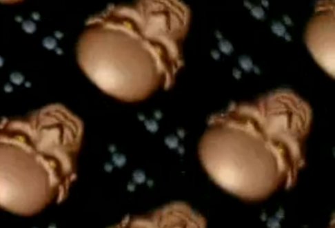
This paragraph describes the Rotozoom effect. A well-known example of this effect is found in "Second Reality" created by the Future Crew.
Fig. 1: Rotozoom in Future Crewĺs "Second Reality" (Assembly, 1993)
We will create a rotozoom like the one shown in figure 1. In essence it is a tiled texture, filling up the screen. Once the scene starts, variables change, moving the tiled image closer and further away from the user; slowly rotating and spinning, creating a dazzling effect.
The rotozoom implemented by this article rotates around the Z-axis and is able to zoom in and out.
Approach
Using figure 2 we discuss the approach taken to creating a fullscreen rotozoom. There are a number of variables that come into play when visualizing this effect. First of all, there is an angle beta that describes the rotation of the rotozoom. Second, there is a zoom factor we shall call rho. Lastly the image that is used has a certain width and height.
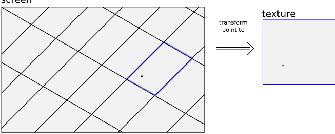
Fig. 2: Transformation from screen- to texture-space
Knowing these variables, we try to devise a method to translate any given point on screen (x,y) to a point inside the texture so we know the colour to display at that position. In our example, this is repeated for every point on screen, resulting in the illusion of a rotational zoom.
From screen- to texture-space
To understand the math below, a small more humanly readable outline is provided of the steps taken to determine which point on screen is at what location in the texture.
1. first translate the (x,y) coordinates into their partial polar counterparts (r,theta);
2. second, reverse the rotation by subtracting the rotational angle from the partial polar coordinates we found;
3. using the new angles, find the unwrapped (u,v) location in texture-space;
4. adjust the coordinates according to the zoom factor;
5. because the texture is tiled, wrap the values to the width and height of the texture.
The following paragraphs show you how to do this using a point for point approach.
Translate
First of all we translate the coordinates from (x,y) to a partial polar representation. The polar coordinates system presents coordinates using radius and angle: (r,theta). Using the formulas below we can perform this translation.
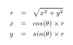
Since we know x and y we can also determine sin(theta) and cos(theta) using:
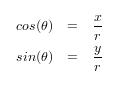
The "partial polar" representation of coordinates has been mentioned a few times now. Instead of performing an inverse- cosine or sine operation to truly retrieve the value of theta, we shall let them remain in their current state. Even without having the exact value, there are formulas that will help us out as shown in the next paragraph.
Reverse
To move the points (x,y) into texture space we have to reverse the rotation that is done to texture space that have resulted in their screen space coordinates.
Imagine that (x,y) has been rotated beta radians with respect to texture space. If we want to calculate the original point in texture space, we apply the reverse operation to the coordinates. This is done by modifying cos(theta) and sin(theta) that has been retrieved in step one. We use the following formulas:
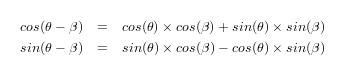
These could also be expressed in matrix calculations, but for the simplicity of this article we shall not.
Wrapping up
To move the points into texture-space we calculate cos(theta - beta) and sin(theta - beta). We can then re-use the formulaĺs from step one, to determine the original texture coordinates. This is also the spot where the zoom factor comes into play:
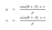
Unfortunately these coordinates do not take into account the limited dimensions of the texture that is being displayed. We still need to wrap the coordinates into something acceptable.
Once all steps above have been executed, we have successfully moved our screen-coordinate back into texture-space. The program then reads the colour available at the location within the texture and applies lighting to it. This is explained in the next paragraph.
2.2 Phong shading
This paragraph explains the "Phong shading" [1] lighting model used in this article. It is a very basic, popular lighting model. Its popularity stems from the algorithmĺs relatively light computational expenses.
The Phong shading model consists of a number of elements. First of all, there is an ambient component. This is the base colour for all elements in the scene and expresses the light emitted by light sources that are too far away to be influenced by position, but strong enough to influence the scene.
The remaning diffuse- and specular light components depend on the position of the point that is being lit with regards to the lights in the scene, they are therefore calculated separately for each light in the scene.
The diffuse component expresses the colour intensity of each light that hits a certain point in the scene. In some scenarios, the diffuse lighting is also influenced by shadows, however, we shall not worry about this ľ after all, weĺre only lighting a flat surface.
Lastly, the specular component expresses the sheen that is left on objects when the materials they are made of, are reflective in nature. A chrome ball would have a high specular constant while a piece of dry concrete would not.
Letĺs continue to the mathematical model used to express these components. The equations below contain ka, kd and ks, they are constants that determine the amount a certain component takes part in the equation and are defined per material that is inside the scene. We only have one material, so we can suffice by defining them only once. The intensity and color of light is determined by ia, id and is.
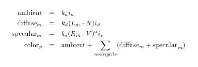
The remainder of the terms used in the model are Lm which is the direction vector from the point we are lighting to light m. N is the surface normal, we will do some magic with this vector when we talk about bump mapping. The terms used in the specular component are: Rm for the reflection ray from light source m over N. The specular component is dependent on the angle from the point to the viewer, V expresses this vector by being the vector that points from the point that is being lit, up to the viewer. Finally, a is a constant that determines the reflectance of surface m.
2.3 Bump mapping
Bump mapping [2] is a technique that has been developed in the late eighties and found its way around the graphical landscape. It allows meshes to have a great amount of detail by altering the surface vector depending on the pixel it is on using a texture lookup instead of addition polygons. In its early days, this technique was popular in ray tracing engines, however, as computers became more and more powerful the transition to real-time renderings was inevitable.
There are a number of ways to create a bump map, we shall create ours using a normal map. The following paragraph explains what that is and how they work.
What is a normal map?
A normal map, in our case, is a two-dimensional array containing vectors. These vectors describe the normal for a specific point on screen or on a mesh. When calculating color values using the Phong shading lighting model, instead of using the surface normal, we determine the position in the normal map that contains surface information for that specific pixel and use that value for our lighting information.
In our example, the vector value in the normal map, maps to a rotating surface. Therefore, our normals should be rotated accordingly. For this, we use the same formulas used for the screen- to texture-space calculations, the adjustment to the angle is -beta.
Normal maps, like textures, are often stored as an image file. The RGB components of each pixel represent the vector components (x,y,z) of the normal at that specific pixel. Figure 3 shows an example of a texture and normal map that was created for it.
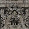
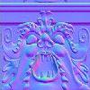
Fig. 3: A texture of a gargoyle and its normal map [3]
Combining the texture with the normal adds an immense perceived depth. The performance hit for this is much lower than creating a model with such incredible detail. This technique is being used a lot in current generation graphics, providing life-like imagery for a next to nothing cost.
3 Implementation
The implementation uses C++ with SDL and the image library extension, for easy per-pixel access. All the renderings you see are done on a software level, there has been no use of wide-spread APIs like OpenGL or DirectX that have these capabilities built-in. This decision was made to make it more clear how the concepts translate to a naive implementation ľ naive because the implementation is straightforward as it has been crafted for educational purposes.
3.1 Flow
This section describes the flow the application goes through to create our bump-mapped rotational zoom as seen in figure 4.
1 // variables
2 L         = collection of lights and lighting information
3 normalMap = 2d array containing the normal map
4 texture   = 2d array containing the texture
5
6 // for every pixel on screen
7 for y from 0 to height:
8    for x from 0 to width:
9
10        // rotozoom
11        (u, v) = texture_location_transform(x, y)
12        u = wrap(u, width)
13        v = wrap(v, width)
14
15        // lighting
16        N = normalMap.vector_at(u, v)
17        Nrot = screen_location_transform(N)
18
19        C = texture.color_at(u, v)
20        rgb = calculate_lighting(L, Nrot, C, x, y)
21
22        // write
23        draw_pixel(x, y, rgb)
24
25    next x
26 next y
Fig. 4: Rotozoom pseudo-code
The pseudo-code has a number of assumptions:
1. a collection of lights has been initialized beforehand, they are now passed to the code;
2. the normal map and texture image are fed into the code and can be queried for information at a position (u,v) where u and v are between zero and the width and height of the texture respectively.
3. the normal map returns a vector with three components (x,y,z) ranging between zero and one;
4. a three component RGB value is returned by the texture map when queried.
The components range from a value between zero and 255.
For every pixel on the screen the original position in texture-space is calculated and wrapped to fall within the boundaries of the texture array. We assume the normal map has the same dimensions as the texture map. After wrapping, the normal and color components are retrieved using the (u,v) position previously obtained. Then, we transform the normal into screen-space by applying the value for cos(theta) and sin(theta) we found in the first step. If we were to skip this operation, the normal would always point to the direction of itĺs original position. Because our rotozoom is rotating this operation is a necessity for a realistic looking result.
The last mathematical operation for the pixel calculates the lighting using the lighting information, the calculated normal, color components and (x,y) position. Finally the pixel is drawn to the screen.
3.2 Screenshots
This last paragraph contains the goodies ľ the screenshots weĺve all been waiting for! It shows a step for step gradual increase in detail.
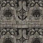
(a) Tiled texture
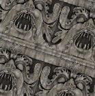
(b) Rotozoom without lighting
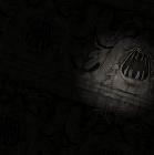
(c) Rotozoom with lighting
(d) Lighting with bump mapping
Fig. 5: Display of step-by-step implementation of new features
4 Conclusion
This article has shown you how to move points from one two-dimensional field to another, by calculating the starting point. The Phong shading model was described; during the rendering of the final lighting a normal map was placed over the rotozoom to create an artificial feeling of relief: a bump map.
By combining these techniques we have created a visually pleasing implementation of the old-skool rotozoom effect.
References
[1] Bui Tuong Phong, Illumination of Computer-Generated Images, (Department of Computer Science, University of Utah), UTEC-CSs-73-129, published July 1973.
[2] Simulation of wrinkled surfaces by James F. Blinn (Caltech/JPL), ACM SIGGRAPH Computer Graphics Volume 12, Issue 3, published August 1978.
[3] Gargoyle texture and normal map courtesy of James Hasting-Trew. Find more on his website at: http://planetpixelemporium.com