Let's be pathetic. :) Linear Algebra! How many useful things lie in this science! How many effects you can create with it! How I like it! How I want to make you like it!
Basically, this says it all. If you still haven't got the point: I give you a course in Linear Algebra, with full explanations. This is the first article from this series, the others will be published in the next issues.
If you are wondering why you should learn Linear Algebra, then read another article of mine, "Economical ways", which is also published in this issue. There I explain how you could profit from all of this and give you two mind-blowing examples of fast proofs of useful things. If you haven't read it yet, then I recommend you to exit from this article and read that one. After reading, you can go here again, of course. We will wait for you with open mind, mouth, heart and soul!
Now, when you have already read "Economic ways" and understood the necessity of Linear Algebra, let's discover what I have prepared for you.
Here is the complete structure of the course:
I. Fields, Matrices, Determinants, Inverse matrices
II. Linear vector space. Systems of vectors. Homogeneous and heterogeneous systems of equations.
III. Euclidean space. Normed space. Orthonormalized bases. Normal and projection.
IV. Linear operators. Eigen values. Operators in real space. Orthogonal operators. Functions from matrices.
V. Elements of analytical geometry: lines, planes etc.
This article covers the first section of this table of contents. (The IVth one will be the greatest, I promise!)
You may think that this is too small, but don't be fooled by this list - and look below! Every entry in this list is very huge, I guarantee!
Now about the source of the covered material. Of course, I wasn't able to discover this myself, or from some online sources, so the origin of all this stuff - is my university lectures. I want to thank my lecturer, V. M. Chubich, for such a great course and such a good and professional manner of teaching!
But of course, you shouldn't think that this article is a simple translation of my copybook with the lectures. No! I claim that 90% of text here has been written by me. In fact, I used the lectures only for giving strict definitions and planning the structure of course (something was dropped out), and nothing else.
So, now you are absolutely prepared for studying, tune up! Welcome to the realm of Linear Algebra!
Fields
First, let's talk about history, let's try to understand why fields are useful, what pre-conditions they had, and only after this let's give a precise definition of them.
At first people discovered numbers, introduced their graphical interpretation and some operations on them (like "+" or "-"). This was an objective decision (however, it was accepted without any committees, there were no committees in this ancient society, as we know, so everything changed step-by-step, not in one minute), practice and life forced them to do it. All of them had to calculate something, farmers - land and harvest, merchants - cash and amount of goods etc.
Then, after dozens of centuries, after the worst periods of The Dark Ages (when almost all experiences of Greek mathematicians had been forgotten), Math began to grow, smart mathematicians appeared in Europe and Asia. This was around the XIV-XV centuries, I suppose.
And many of them realised that they needed something more than simple numbers, Euclid's geometry and all those ancient things. So, Algebra was introduced, where numbers were written as letters, symbols. Only think how convenient this was and how big this step was! For example, one could find a symbolic solution for some task, and then solve different tasks, which have the same structure using the only formula, simply by inserting concrete values instead of symbols. So, now any math education is impossible without algebra.
Now let's go further. Step by step mathematicians started to feel constrained by numbers, they felt that they needed yet something more than simple numbers, and symbols representing them. They thought: maybe there are some objects, which have complicated structure, but we could perform some regular operations with them? How to determine if some class of objects is applicable for using the regular operations on the objects of this class, how to choose correct base operations for such objects? After a long time of trying, the flexible theory of fields and rings was introduced. Rings are similar to fields, except one thing, but let's speak about this later.
So, let's repeat once more: Why are fields useful? Answer: because they define some object-independent structure of spaces, which have the same properties and operations. They show us how to define basic operations for such spaces of complicated objects such a way that we could perform operations on them, which have the similar properties with the regular operations with regular numbers.
Let's give a strict definition of a field.
DEFINITION
A field is a set of elements, F={a, b, ...}, for each of them two operations are defined: "sum" and "multiplication", and the following axioms apply:
A. Axioms of sum.
1. a+b=b+a for every a,b from field F
2. (a+b)+c=a+(b+c)
3. There is a "null element", let's write it as  .
Its property is: a+=a for every a from F.
.
Its property is: a+=a for every a from F.
4. There is an inverse element, which has the following property:
a+(-a)=, where (-a) is an inverse element for a.
B. Axioms of multiplication.
1. a*b=b*a for every a,b
2. (a*b)*c=a*(b*c)
3. There is a "unit element", let's write it as 1. Its property is: a*1=a for every a from F.
4. There is a reciprocal element for every element in this field. Its property:
a* =1, where means reciprocal element. (a<>)
C. Mixed axiom
1. a*(b+c)=a*b+a*c
"+" and "*" operations are algebraical. This means that they are: binary (take two operands), one-to-one, self-contained (the result of the operation is also an element from this field).
END OF DEFINITION
What is one-to-one in terms of field? The operation is one-to-one when:
1) We can compute it from any two elements of the field.
2) Otherwise, any value of the field can be derived from using this operation on two values (we don't know them in general, simply we know that they exist) from this field.
On guy asked me today (20th July, 2001) if there is any operation that isn't one-to-one. My answer: of course there are such operation(s)! For example, division. It can't be used as one of the two main operations in the field! Why? Look, it doesn't fulfil the 1) condition of the definition of a one-to-one operation. For example, consider two values from field, 1 and O. Can we divide them by each other? In one case we can (0/1), in another (1/0) - can't. So, we cannot compute the operation from all elements of the field, so it isn't a one-to-one operation, and can't be used in the definition of the field.
But of course, don't get me wrong, in the field of real numbers we can use division as well as
other operations. Simply in this case in the definition of the field of real numbers we get
multiplication and sum of the real numbers as two primary operations, and division could be
derived as b*, this is equal to b/a, where is the
reciprocal value. And since all elements of field except have reciprocal
elements, and multiplication is defined for all elements, division is possible.
So, we simply shouldn't define normal division as one of the two main operations in the field, "sum" or "multiplication" (look below why do I write them in brackets), but can use it as a derived operation from multiplication.
Now, when you know the definition of field, it's time to speak about the meaning of this. First, why are the operations in the definition in quotation marks, "sum" and "multiplication"? Answer: because we don't do any suggestions about their nature. This isn't sum and multiplication from regular math. Well, they are, but only in concrete cases, when we agree that in the field of algebraic numbers we will use these two regular operations. Also note, that the elements of the field don't have to be numbers! That is why we write "elements" instead of "numbers".
Now a little example.
We have a set of natural numbers with two regular math operations defined. Question: is this set a
field?
Answer: no. Think why then read the solution.
Solution: From axiom B4 we know that there should be a reciprocal element for every element of
this field which also lies in this field. Good. Let's take any element a from this field
except 1. Then let's try to find its reciprocal value. It will be 1/a. We see, that the reciprocal
value doesn't lie in the field of natural numbers but in the field of rational numbers. Axiom B4
isn't fulfilled. This isn't a field.
Consequences of the axioms
As soon as the axioms are fulfilled we can prove the following properties. I give a proof only to the first one, deduce the others by yourself, it is very easy and it's a good task to solve.
1. There is only one null element in field F.
Proof: Let's suppose there are two null elements,  and
and
 .
.
We know that a+=a. From the other side
a+=a (*).
Now let's place instead of a in an expression (*):
=+=|axiom A1|=+=|axiom A3|=.
We see: =.
2. There is only one inverse element in field F.
3. -(a+b)=(-a)+(-b)
4. There is only one unit element in field F.
5. There is only one reciprocal element in field F.
6. 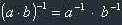
7. *a=
8. (-a)=(-1)*a.
Don't forget that the unite element 1 and the null element aren't the
numbers 1 and 0 in general!!!
Examples of fields
1) All real numbers are a field.
2) All complex numbers are a field.
3) Natural numbers aren't a field.
These are the most useful examples of fields.
Now a couple of words about rings. Rings are similar to fields, BUT the "multiplication" in them isn't commutative! And the next chapter will be dedicated to one example of a ring: the ring of matrices.
Matrices
Let's talk a little before we will give definitions, just like this was with fields. Again, why matrices, what are matrices? If to speak non-strictly, a matrix is a table of numbers. More, you are already familiar with them. All those arrays in programming languages are similar to matrices. But why should we use them? You know why to use arrays in programming - to store some data, etc. But in mathematics matrices are used in another way. A matrix - isn't an array! For example, we can't multiply or add arrays, can we? But these operations are defined for matrices. A long time ago people noticed that some long expressions can become smaller, if they are written in small tables (matrices) and then the original expression is derived by some operations on these matrices (such as addition, multiplication etc). Of course, it's interesting what operations are possible with matrices, we will look at them. But matrices aren't used only to simplify some expressions. Generally, matrices in Linear Algebra are like numbers in school algebra, it is impossible to get anything without them. With matrices you could solve big systems of linear equations (mostly systems, where the number of equations isn't equal to the number of variables), and this is a very serious thing in L.A. You will discover these systems almost everywhere in practical tasks.
So, deep and strong knowledge of matrices is required for further learning! Let's start!
DEFINITION
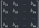
A matrix is an aggregate of elements A[ij] taken from field F which are written in the form of a table, which has the dimension MxN.
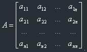
Let's agree to write the matrices starting with capital letters: A, B etc, and the elements of a matrix starting with lower-case letters: a11 etc.
Note that the first index in the element is the number of the row and the second is the number of the column! When we write that the dimension of the matrix is m x n, then we suppose that it has m rows and n columns!
If m=n then the matrix is called a square matrix. Otherwise it is called a rectangle matrix.
Operations on matrices
1) If two matrices A and B have equal dimensions then they are comparable. A=B applies if and only if aij=bij for every i=1..m, j=1..n. aij are elements of A, bij - of B.
2) The matrix C is called a multiplication of matrix A on number c when cij=c*aij, i=1..m, j=1..n.
3) Let's suppose that matrices A and B have the following dimensions:
A: m x n; B=n x k.
Then we can introduce a multiplication of matrix A on matrix B.
Matrix C is called a multiplication of matrix A on matrix B when
cij=ai1*b1j + ai2*b2j + ... + ain*bnj
C - equal to A*B - has the dimensions m x k.
Note that the middle index is "eaten" by multiplication. I mean if A is 3x4 and B is 4x5 then A*B will be 3x5.
A little example of multiplication:
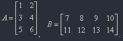
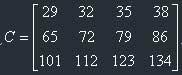
C=A*B. C will be 3 x 4
c11=1*7+2*11=29
c12=1*8+2*12=32
c13=1*9+2*13=35
c14=1*10+2*14=38
c21=3*7+4*11=65
c22=3*8+4*12=72
c23=3*9+4*13=79
c24=3*10+4*14=86
c31=5*7+6*11=101
c32=5*8+6*12=112
c33=5*9+6*13=123
c34=5*10+6*14=134
So:
The memorizing rule for multiplication of matrices is: The matrices are multiplied "a row by column": The first element of the result is the sum of the multiplications of the elements of the first row of the first matrix on the first column of the second matrix and so on.
The implementation of multiplication
Here is the simplest program for multiplication of matrices A and B, in general case. Matrix A has dimensions m x n, B - n x k.
type_of_el* mult(type_of_el* A, type_of_el* B)
{
int i,j,l;
type_of_el* C = new[m][k];

	for (i=0; i<m; ++i)
	{
		for (j=0; j<k; ++j)
		{
			C[i,j]=0;
			for (l=0; l<n; ++l)
			{
				C[i,j] = C[i,j] + A[i,l]*B[l,j];
			}
		}
	}
	return C;
}
Small note: you must use the additional matrix C for result, because multiplication needs the previous values from both matrices!
Of course this isn't optimal, and can be implemented only in some purely mathematical programs. So, the optimisation note: since the most widespread usage of Linear Algebra in the computer world is 3D graphics, we can optimize multiplication following this simplification, which is true for 3D graphics:
All matrices are either 3x3 or 4x4 (later I will explain why we need 4x4 matrices), and are square matrices, which is obvious from their dimensions.
So, as we know that we will deal with 4x4 matrices (most of the time), we can write a faster function (however, I will demonstrate the idea only for 3x3 matrices, because the 4x4 function will have 16 lines, while this has only 9, but the idea is clear: we unloop three cycles into a non-iterating procedure):
procedure mult3D(var A:_3Dmatrix; var B:_3Dmatrix; var C:_3Dmatrix);
begin
  c[1,1]:=a[1,1]*b[1,1]+a[1,2]*b[2,1]+a[1,3]*b[3,1];
  c[1,2]:=a[1,1]*b[1,2]+a[1,2]*b[2,2]+a[1,3]*b[3,2];
  c[1,3]:=a[1,1]*b[1,3]+a[1,2]*b[2,3]+a[1,3]*b[3,3];

  c[2,1]:=a[2,1]*b[1,1]+a[2,2]*b[2,1]+a[2,3]*b[3,1];
  c[2,2]:=a[2,1]*b[1,2]+a[2,2]*b[2,2]+a[2,3]*b[3,2];
  c[2,3]:=a[2,1]*b[1,3]+a[2,2]*b[2,3]+a[2,3]*b[3,3];

  c[3,1]:=a[3,1]*b[1,1]+a[3,2]*b[2,1]+a[3,3]*b[3,1];
  c[3,2]:=a[3,1]*b[1,2]+a[3,2]*b[2,2]+a[3,3]*b[3,2];
  c[3,3]:=a[3,1]*b[1,3]+a[3,2]*b[2,3]+a[3,3]*b[3,3];
end;
Err, why not C? Don't get angry, Pascal is also useful sometimes. ;) And in this procedure there are only three Pascal-specific lines.
Properties of matrices
1. A+B=B+A
2. (A+B)+C=A+(B+C)
3. (a+b)*A=a*A+b*A, where a and b are the elements of the field.
4. a*(A+B)=a*A+b*B
5. A+A=2A
6. (-a)*A=-(a*A)
7. -(-A)=A
8. A*B <> B*A (!!!)
9. A*(B*C)=(A*B)*C
10. (A+B)*C=A*C+B*C
11. C*(A+B)=C*A+C*B
Remember the 8th property!
But also remember the 9th property. It gives us a great mechanism to use in practice (3D transformations in our case). If we write some transformation in the form of a matrix and have to perform several consecutive transformations on our object, and each transformation has its own matrix, the resulting transformation matrix will be a multiplication of all matrices, in random order (if the number of matrices is more than 2), only keeping the last and the first matrices at their places! So, we have to calculate one matrix only once a run of the program, and then use it when we need to do the transformation.
Due to the fact that the multiplication of matrices isn't commutative, we can't say that matrices form a field. (But they form a ring instead.)
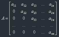
Diagonal matrices
A square matrix is called diagonal when all its non-diagonal elements are equal to zero. "Diagonal" means main diagonal, it goes from the upper left edge to the bottom right one:
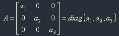
If all diagonal elements in a diagonal matrix are equal to 1, then the matrix is called a unit matrix, and usually is written as I or E.
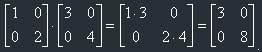
The sum and product of two diagonal matrices are also diagonal matrices and their diagonal elements are equal to, respectively, the sum and product of their diagonal elements:
Diagonal matrices could be implemented in 1D arrays, for a n x n diagonal matrix we need an array of n elements.
Transposition of a matrix
The matrix ![]() is called the transposed matrix of the square matrix A
if the following conditions are fulfilled:
is called the transposed matrix of the square matrix A
if the following conditions are fulfilled:
The matrices have equal dimensions and  =
= , where i,j: 1..n
(n is the size of matrix),
, where i,j: 1..n
(n is the size of matrix),
- elements of matrix ![]() , - element
of matrix A.
, - element
of matrix A.
The transposition of a matrix may be treated as an operation on the matrix.
In this tutorial I always will write the transposed matrix for matrix A as ![]() .
.
Implementation (or why you are studying this)
In fact, if you look at A and ![]() you will notice the following rule:
the transposed matrix is a symmetry around the main diagonal. This flows from condition
=.
you will notice the following rule:
the transposed matrix is a symmetry around the main diagonal. This flows from condition
=.
But this isn't all. When you will code it in a real project, mind the following: to perform
the transposition you don't have to move any elements in memory! Let's suppose that we have
to calculate ![]() *A, and we have a function
*A, and we have a function
(type_of_el*) mult(type_of_el* A, type_of_el* B),
which multiplies matrix A with matrix B and returns a pointer to the new matrix, the product. Suppose we have a case when we need to perform the multiplication of some matrix not on another matrix B, but on the matrix, which has to be derived from B by transposing. But we don't want to transpose it, right? So, you simply have to introduce a flag in header of function, which will "turn" the condition that matrix B should be "faked-transposed" in time of multiplication. Of course, you should introduce another flag, which will show that matrix A should be transposed, if needed. And then in implementation we simply change the order of multiplication of elements! Example:
(type_of_el*) mult(type_of_el* A, type_of_el* B, BOOL isBtransp)
{
type_of_el* C = new[n][n];  //transposed matrix should be square matrix
int i,j,l;

	if (isBtransp)
	{				// when B needs to be transposed
		for (i=0; i<n; ++i)
		{
			for(j=0; j<n; ++j)
			{
				C[i,j]=0;
				for (l=0; l<n; ++l)
				{
					C[i,j] = C[i,j] + A[i,l]*B[j,l];
					//because b'ij=bji!
				}
			}
		}
	} else
	{				// when B doesn't need to be transposed
		for (i=0; i<n; ++i)
		{
			for(j=0; j<n; ++j)
			{
				C[i,j]=0;
				for (l=0; l<n; ++l)
				{
					C[i,j] = C[i,j] + A[i,l]*B[l,j];
				}
			}
		}
	}
	return C;
}
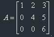
Triangular and trapezoidal matrices
What is a trapezoidal matrix? It means the following:
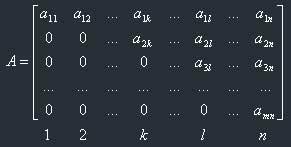
k, l, ... are natural numbers which lie in [1, n]. Wanna example to simplify understanding? Here it is:
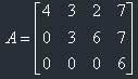
This is a trapezoidal matrix, here k=2, l=4, m=3, n=4.
The nulls in such a matrix are similar to a perverted "trapezium".
I've found a simple rule for understanding this: in a trapezoidal matrix the following applies: If we see that on the n-th row that there are k zeroes from the beginning, then in all following rows there should be more zeroes from the beginning of the row; and this should apply for any row (except the last, of course).
Triangular matrices are a bit easier, it means:
So, as we see, a triangular matrix should be a square. Also it's obvious that there are individual cases of trapezoidal matrices.
Example:
Determinants
We can treat a determinant as some function of a matrix which "determines" it. The determinant, basically, is a number. Simply a number. However, this number can show us some of the properties of the matrix (for example, could we find an inverse matrix or not - but later about it), so determinants are very important. Where are they used? First, they are used for finding eigen values (but we won't talk about them, unless you will ask me to cover them in the next chapters) of the matrix. Eigen values are very important in some theoretical (not practical) areas of Linear Algebra, e.g. for deep exploration of linear operators, the theory of Jordan's normal form. So, as determinants lie in basis of all this stuff, they are important.
But this isn't the only area of using determinants. Determinants, just like matrices, could "squeeze" some huge formulae in one basic "block". For example, the equation of a nD plane (it could be 2D, 3D, how much you want), if we know the required amount of points which lie on this plane, is written in the form of determinant, by the way. As you see, planes are very important in graphics, so you should know determinants to use planes, which are defined only by points, which lie on them.
Let's suppose that A is a square matrix, its size is n x n, and its elements have the names aij and have been taken from field F; i,j: 1..n.
Let's write all possible multiplications of n elements of a matrix, where in every line and every column of the matrix only one element is taken. Because aij are taken from field F, their multiplication is commutative, so we can sort each of these multiplication groups by the number of column. As a result we will get multiplications in the following form:
ai1,1 * ai2,2 * ... * ain,n (1)
where i1, i2, ... represent the numbers of rows after the exchanging of factors.
Now a little definition: The inversion (or disorder) of sequence i1, i2, ... is such a disposition of elements where the higher index stands before the lower index. Let's call the number of inversions N(i1,i2,...in). A few little examples:
1) N(1,2,3)=0
We see that all indexes are sorted, so the number of inversions is zero.
2) N(2,1,3)=1
Here we have only one inversion, look: 2>1 but it stands before 1.
3) N(3,2,1)=3
There are 3 inversions:
First: 3 and 2
Second: 3 and 1
Third: 2 and 1
Let's agree that we will mark groups (1) with a sign, which depends on the number of inversions in the sequence i1, i2, ... If the number is even, then the sign is "+", if odd - the sign is "-".
DEFINITION: The determinant of the square matrix A is the sum of all possible products (1) where each summand is taken with the sign.

It's easy to understand the last formula, it gives us +1 when the number of inversions in this group is even, and (-1) when this number is odd.
It is obvious that the number of summands for the determinant of matrix A(n x n) is n!
(n factorial).
For those who don't know what factorial means: n! = 1 * 2 * 3 * ... * n, 0! = 1
This comes from combinatorics.
The determinant of matrix A is written as det A, or the matrix is written in simple vertical brackets:

Let's find formulae for the determinants of 2 x 2 and 3 x 3 matrices.
1)
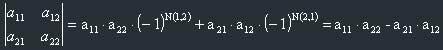
2)
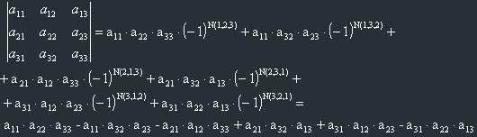
We can derive a memorizing rule for determinants of 3 x 3 matrices:
Let's divide the products of elements belonging to a 3 x 3 matrix into 2 groups:
1) Imagine the main diagonal of matrix (a11, a22, a33). This group, I mean a11*a22*a33, will belong to the first group. Then imagine two "triangles", built from numbers, the first one is (a21,a32,a13) and the second is (a31,a12,a23). We see that one of their sides is parallel to the main diagonal. These two products ((a21*a32*13) and (a31,a12,a23)) also belong to the first group.
2) Imagine the secondary diagonal (a31,a22,a13). Let it belong to the second group. Now imagine two other triangles: (a21,a12,a33) and (a11,a32,a33). One of their sides is parallel to the secondary diagonal. They also belong to the second group.
Now the memorizing rule is the following: In the determinant of a 3 x 3 matrix multiplications belonging to the first group are taken with their original signs, and elements belonging to the second group are taken with inverse signs. This rule is called "rule of triangle".
Example:
A matrix whose determinant is equal to 0 is called a singular matrix.
Now let's look at some properties of determinants.
Properties of determinants
1) det(A') = det(A)
A' means matrix transposed to A.
2) All following properties, which apply to rows (columns), also apply to columns (rows) of matrices.
3) Antisymmetry of columns. If we exchange two columns (rows) in matrix then the sign of its determinant will change on inverse while absolute value won't change.
4) Determinant of matrix, which has two equal rows (columns) is equal to zero.
5) If all elements of row or column in matrix equal to zero, then its determinant is equal to zero.
6) The determinant won't change if we add to some row (column) another row (column), all elements of which are multiplied on the same (arbitrary, but not 0) number.
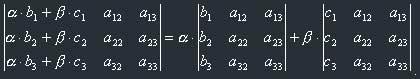
7) Linear property of a determinant.
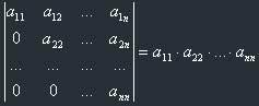
8) The determinant of a triangular matrix is equal to the product of its diagonal elements:
Let's make this working for us!
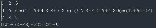
Let's find a determinant of a matrix using these properties: (numbers in comments mean numbers of axioms)
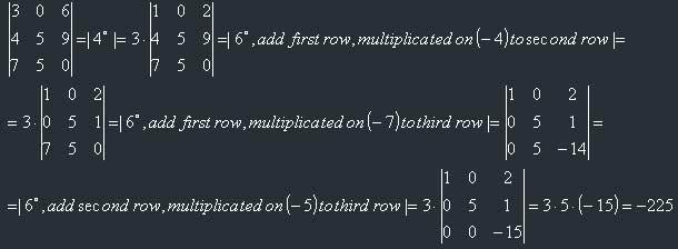
So, our task consists of transforming the matrix of the determinant to triangular form, and then using the 8th property. Note, that for making this task automatic (for yourself or for the computer), you should work with one column at a time! I mean, first you should "make" zeroes below a11, and only then start "make" zeroes below a22, and so on until a(n-1),(n-1) inclusively. This guarantees an automatic solving of the problem.
Of course, this method is quite hard, and for big determinants we could use a more convenient and even more automated way. So:
Laplace's Theorem
To be precise, I won't give you full Laplace's theorem, because you, probably, won't need it too much. In my opinion, everything can be calculated easily using reduced Laplace's theorem, and also it gives a convenient way of programming the calculation of determinants using a computer. And to explain you the full theorem means to write a couple of kilobytes more to me - and several dozens of minutes of thinking to you. So, all of us profit from this. :)
Let's first find out what the term "algebraical complement" means.
The algebraical complement, Aij, of the element aij in the matrix A is the following expression:
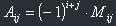 , where Mij means determinant of matrix which comes to hand from the omission of the i-th row, and the j-th column in the original matrix.
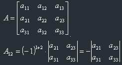
Example: Let's find the algebraical complement of element a12 in matrix A.
Note once more: when I write a matrix in square brackets, I mean that it is a regular matrix, but when I write it in simple vertical brackets, I (and everyone who learns Linear Algebra) mean the determinant of this matrix, i.e. some number. So, the algebraical complement is a number.
And now we know everything to use the reduced Laplace's theorem. So:
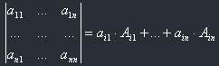
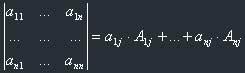
Theorem: Let's choose one row (column) in the matrix. Then determinant of this matrix is equal to the sum of all groups, where each group consists of the corresponding element from the chosen row (column) multiplied with the algebraical complement of this element.
Or, if to write in symbols:
1) in case we've chosen a row, and its number is i:
2) in case we've chosen a column, and its number is j:
Now about tactics: it is obvious, that it's better to choose the column or row where we have the biggest number of zeroes, because in this case the corresponding summands will also be equal to zero.
Example: Let's find the determinant of the following matrix:
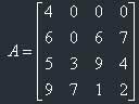
Let's choose the first row. Now, from Laplace's theorem:
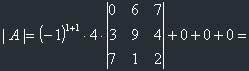
(You see, the last three summands are zeroes because there are three zeroes in the row we've chosen - tactics! ;))
Now let's continue and calculate this 3x3 determinant, again using Laplace's theorem. Let's also choose the first row, because, you see, there is one zero.
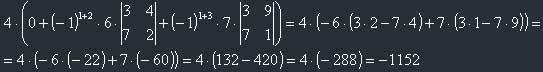
Yes, we've got the final answer! Just imagine how long you can calculate this determinant with the regular method! If you think this isn't correct, then go to MathCAD and get the same there. Also note: for calculation of 2x2 determinants I used a formula, derived a couple of pages above.
Implementation
It is very obvious, that this can be implemented with ordinary recursion. Without any thinking and hacking. In the procedure below I always choose the first row for using in Laplace's theorem. Of course, your procedure could look at the whole array and to find the row or column with the biggest amount of zeroes, and then use this row (column).
float determinant(float* matrix[], int dimension)
{
float temp = 0;
int sign = 1;

	if (dimension>1)
	{
		for (int i=0; i<dimension; ++i)
		{
			temp += sign * matrix[i] * determinant(
				 Complement(matrix,dimension,i),dimension-1);
			sign = -sign;
		}
	} else
	{
		temp = matrix[0];
	}
	return temp;
}
We stop the recursion when the matrix becomes 1x1 (single number) and its determinant equal to this number.
The procedure Complement (which isn't provided) forms a new array by omitting the corresponding row and column (in this example the row number is always equal to 1, and the column number is i (cycling variable)).
In each iteration we change sign, this is the programming approach to calculate (-1)^n.
A matrix inverse to A is such a matrix  that fulfils the following condition:
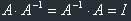 , I is unit matrix.
Since I is a square matrix, A and should also be square; they won't produce
a square matrix otherwise.
Also, we can find the inverse matrix if and only if the matrix isn't singular (det<>0).
An inverse matrix is a very useful thing, and will be used in some transformations. In general, it acts like the "Undo" command.
Now about practical ways of finding the inverse matrix. First, you should know the canonical way; it could be hard, however.
1) Canonical way.
We have the matrix:
Then the inverse matrix will look the following way:
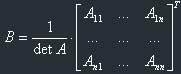
...where Aij are the corresponding algebraical complements of the elements of the matrix. Don't forget about the final transposing of the matrix! I always forget it.
Now example, let's constrain ourselves to a 3x3 matrix (to minimize calculations).

We should find the inverse matrix for this matrix. First, let's find the determinant.
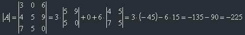
It isn't equal to zero, so it is possible to find the inverse matrix.
Now the next step, to find all algebraical complements (if you still don't understand them, then this example will be good).
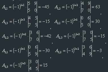
So:
Now let's check, if we find it correctly. For this let's remember the definition of the inverse
matrix: 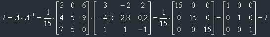
Oh, god! After several hours we have received the correct result!
To be absolutely strict, you should also check if  , because matrix
multiplication isn't commutative, and this condition should also apply. But it's already a home
task for you. :)
, because matrix
multiplication isn't commutative, and this condition should also apply. But it's already a home
task for you. :)
2) Normal way
The concept of this method is:
1) Transform your given matrix, n x n, to n x 2n following the following picture:
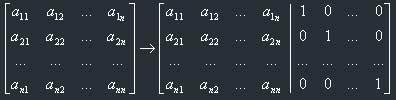
(i.e., complement it with the unit matrix from the right side).
2) Now apply elementary transformations on the rows of the matrix in order to achieve such a form of this matrix that its left half is occupied by the unit matrix and its right half will be the desired inverse matrix. Diagram:
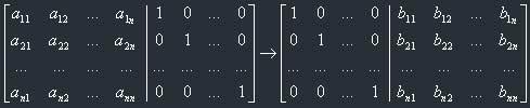
Now this matrix is our inverse matrix:
However, you still don't know one thing - elementary transformations of matrices. Strictly, in this chapter I shouldn't give them, because they can be introduced only when linear vector space has been introduced, and some other stuff has been learned. But, to actually perform this algorithm, we still need them, so here they are:
Elementary transformations of matrix:
1) Multiplication of one row with a fixed number (but not zero!).
Example:
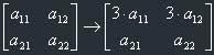
Here we've multiplied the first row with 3.
2) Exchanging of row with row.
Example:
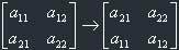
Here we've exchanged the first row with the second row.
3) Addition of all elements of one row the elements of which have already been multiplied with
the desired fixed number (which isn't zero) to the corresponding elements of another row.
Example:
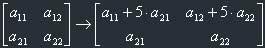
Here we've added the elements of the second row, multiplied with 5, to the elements of the first row.
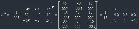
Now an actual example of calculation of the inverse matrix by this method. Let's take the same matrix as in the previous method and then compare them.
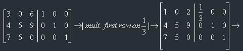
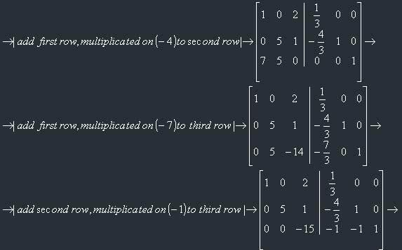
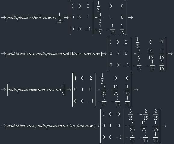
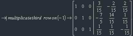
So, now we've got the inverse matrix:
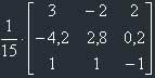
I've divided each element by 15 and placed 1/15 before the matrix for further convenience in calculations.
As we see, the matrix is the same as we got with the first method. But this method is faster.
If you still can't get how exactly we've found the way of transforming the original matrix to the unit matrix then hint: this task is divided in three subtasks:
1) Transform our matrix to a triangular one, using this scheme: First of all, exchange the rows in such a way that after exchanging we get a number which isn't equal to zero at the leftmost top position in the matrix. Then using transformations types 1) and 3) make such transformations that below element a11 there will be only zeroes in this column. Then do the same with the following columns. So, as a result you will get a triangular matrix.
2) Then we should transform our triangular matrix to a diagonal one, using the same techniques, but starting from element ann, from bottom to top. We will get a diagonal matrix.
3) Now we should get the unit matrix from this diagonal matrix. And this is very simple. Use the 1) property to achieve this by multiplying our rows with the reciprocal element of the desired number.
All this steps can be seen very clearly in the example I give above.
Matrix equations
Matrix equations are very simple and look like this: A*B=D*E, and the task is to find, for
example, matrix A. And here we, of course, should use inverse matrices. Let's solve this
particular task. Let's multiply both parts of our equation on  , from the
right side. We will get:
, from the
right side. We will get: 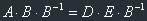
Because  and
and  , we get the final answer:
 .
.
Note: if you place the inverse matrix to the right end of the left part of the equation, you must place this matrix also on the right end of the right part. Matrices aren't numbers, and we will get a wrong answer otherwise!
In closing
So, now it's time to say goodbye. But not farewell, of course! We will meet in the next issue of Hugi where I will offer you next chapter of this article series. I wait for your comments, suggestions and feedback, of course. You can ask me any questions about the subject, I will try to answer them. My email is iliks@chat.ru (or iliks@mail.ru).
Does anyone want to see all things above proved? Or maybe someone wants to prove all of this himself? :) Of course, if you want to see every theorem and statement proved, simply say this to me, I will try include them. But then this won't be article but a BOOK! I supposed that you would be able to use all this things without proving, only with the definition.
By the way, two days ago I read this phrase: a computer scientist programs to learn, but a software engineer learns to program. So, I've taught you a bit, now let's go to implement the methods of L.A.! Now!
iliks was with you.
(C) 2001. Ilya Palopezhencev