I learnt the things that I have learnt while experimenting with Mathematica at university. Mathematica is a wonderful program created by people who undoubtedly know this stuff; the packages I use to derive these approximations were used to deduce the very same formulas that Mathematica uses to compute transcendental functions. Some more information was deduced by looking at the source code for the GNU C library.
The fundamental property of Taylor's polynomials, as Adok has probably explained in his article (which I did not read...), is that the nth-order polynomial for f(x) computed around x0 not only has the same value as f(x) for x=x0, but it also shares the first n-1 derivatives. This means that the polynomial "knows" something about how the function behaves near x0 too.
But what if the polynomial's knowledge of f(x), instead of being focused on x0, was spread around n values near x0? What we obtain is known as interpolation: of course we'll lose exact derivatives, because the n coefficients of the polynomial are determined by n constraints (of which n-1 are derivatives for Taylor's polynomials), but we will be able to do a better estimate of the range of x for which the error is sufficiently low.
Basic (and very rough) interpolation was often done a few years ago in 4kb or 256byte intros. For example, one could think to define sin(x) between -Pi and Pi like this:
- if it is < 0, compute -sin(-x)
- if it is > 0, it "is" the parabola that touches (0,0) (Pi/2,1)
and (Pi,0)
You can see that the formula is 4 x (Pi-x) / Pi^2. In this case it is easy because we have both the roots of the parabola, that is, 0 and Pi. One can however derive a general formula for interpolation, and we'll do that later.
How does the interpolation behave (in all the graphics, red is the approximation and blue is the original)?
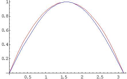
...decently. The maximum error is 0,05 = 3/4 - Sqrt(2)/2 so you can guess that the interpolation is fine as long as your scanlines are shorter than 20 pixels. However this approximation has a very nice feature for a sin(x) interpolation -- namely, that sin(Pi/4) = sin(3 Pi/4), which is very important because people expect lines with a 45 degrees inclination to be perfect.
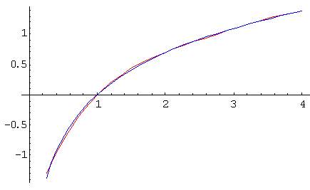
Now say you want to interpolate the logarithm with a cubic, which gives us 4 points to choose. It might make sense to make our polynomial be exact for powers of 2, so we pick .25, 1, 2 and 4. A little Mathematica black magic gives us the polynomial (italic is what I typed):
FInterpolate[f_, x0_] := InterpolatingPolynomial[
            Map[{#,f[#]}&, x0], x];

FInterpolate[Log, {.25, 1, 2, 4}]


Out[2]= -1.38629 +
       ( 1.84839 +
       (-0.66014 +
         0.145231 (x-2)) (x-1)) (x-0.25)
(FInterpolate is needed because InterpolatingPolynomial accepts x/y pairs rather than a function to interpolate. Those of you that know LISP might be illuminated if they read Map as Mapcar and the postfix & as Lambda.) The result is quite poor, as you can see, but Mathematica gave us a hint on how to build the polynomial.
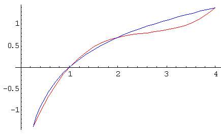
The key observation is that it is of the form log 0.25 + something * (x-0.25), with the something having exactly the same form. So we can obtain it recursively -- again, LISP freaks will feel at home :-) -- as
P(x0) = f(x0) + (Interpolation of (f-f(x0))/(x-x0) in the other points)(x-x0)
We interpolate (f-f(x0))/(x-x0) instead of simply f because we have to "undo" the effect of the linear transformation that constrains P(x0) to be f(x0).
Here is the C implementation of the algorithms. It replaces the y vector with the magic numbers that Mathematica found, and which can then be passed to compute:
   void
   interpolate (float *x, float *y, int n)
   {
     int i, j;
     for (i = 0; i < n; i++)
       for (j = i + 1; j < n; j++)
         y[j] = (y[i]-y[j]) / (x[i]-x[j]);
   }

   float
   compute (float *x, float *y, int n, float x0)
   {
     float f = y[--n];
     while (n-- > 0)
       f = f * (x0 - x[n]) + y[n];

     return f;
   }
Note that good interpolation is harder to do than simply picking a Taylor polynomial. For the sine we were lucky, but it can be difficult to find a good set of interpolation points, and indeed we did not guess it right for the logarithm. One could think of complex algorithms which use more points where the function looks "less like" a polynomial... instead, the answer is quite simple: for every degree n and range in which to interpolate, it turns out that there is a set of x which gives a MINIMAX interpolation. That is, an interpolation whose MAXimum absolute error can be proved to be MINImum.
What's best, is that these x are all algebraic and are the root of a polynomial -- a Chebyshev polynomial of the first kind, written Tn(x). These are polynomials with some interesting properties including this: Tn(x) = cos (n arccos x). Curious, huh? They also look nice:
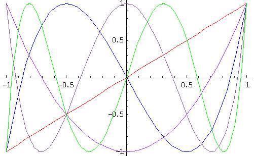
They are obtained recursively with these formulas
Tn(x) = 2x Tn-1(x) - Tn-2(x)
T0(x) = 1
T1(x) = x
Using the roots is fine if your function has x in the range from -1 to 1, else you'll have to pass them through a linear transformation. This C program does that after having used the recurrence relationships to get Tn(x) and found the roots with Newton's method.
  /* A generic polynomial solver using Newton's method, with
     the given tolerance.  Assumes that the n roots are all real. */
  void
  polysolve(float *f, float *x, int n, float tol)
  {
    float oldx, *b, y, d, *tmp;
    int i;

    b = alloca(sizeof(float) * (n + 1));
    do {
      *x = 0.0;
      do {
        oldx = *x;

        /* Divide the polynomial by x-x0 in b(n), get the value in x=x0
           in y and the derivative in d. This is called the nested
           multiplication algorithm and recalls high school's Ruffini's
           rule. */

        b[n] = 0.0;
        b[n-1] = d = f[n];
        for (i = n-1; i > 0; i--) {
          b[i-1] = *x * b[i] + f[i];
          d = *x * d + b[i-1];
        }
        y = *x * b[0] + f[0];

        /* We must not divide by zero even if x got exactly on a maximum
           or minimum */
        if (fabs(d) < 1.0e-10)
          *x += tol * 2.0;
        else
          *x -= y / d;
      } while (fabs(oldx - *x) >= tol);

      /* The results of division by (x - *x) are already in b; this
         is the polynomial for which we are going to find the next
         root. */
      tmp = f;
      f = b;
      b = tmp;
      x++;
    } while(n-- > 0);
  }

  /* Compute the roots of the n-th Chebyshev polynomial,
     and deduce the points in which an interpolation in [a,b]
     should be done */
  void
  chebyshevt(float *x, int n, float a, float b)
  {
    float *f[3], *g;
    int i, j;

    f[0] = alloca(sizeof(float) * (n + 1));
    f[1] = alloca(sizeof(float) * (n + 1));
    f[2] = alloca(sizeof(float) * (n + 1));

    /* Initialize the polynomials */
    for (i = 0; i < n; i++)
      f[0][i] = f[1][i] = f[2][i] = 0.0;

    f[0][0] = f[1][1] = 1.0;

    for (i = 2; i <= n; i++) {
      /* Compute the recurrence relationship */
      f[2][0] = 0.0;
      for (j = 0; j < n; j++) {
        f[2][j+1] = 2.0 * f[1][j];
        f[2][j] -= f[0][j];
      }

      /* Rotate the arrays */
      g = f[0];
      f[0] = f[1];
      f[1] = f[2];
      f[2] = g;
    }

    /* Now the polynomial is in f[1] */
    polysolve(f[1], x, n, 1.0e-10);
    for (i = 0; i < n; i++)
     x[i] = (a+b)/2 + (b-a)/2 * x[i];
  }
Computing the interpolation coefficients is now very easy:
  float x[5], y[5];
  int i;
  chebyshevt(x, 5, .25, 4);
  for (i = 0; i < 5; i++)
    y[i] = ln(x[i]);

  interpolate(x, y, 5);
Here is a sine and a logarithm interpolated with fifth-order Chebyshev polynomials. The maximum error is not only minimum, it is indeed quite small (0.001 for the sine)...
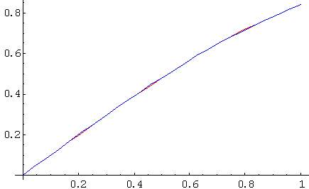
The interpolation coefficients in x and y can be computed once and stored beforehand, or precomputed at run time. Newton's method will usually run for less than 10 iterations, so the time to compute the x coefficients will be negligible.
Now, we are almost done -- only a few tricks.
The first trick is to take advantage of the nature of the function. The trick we had used of interpolating the sine for x>0 only, and use the sin(-x) = -sin(x) identity, still holds when using these techniques.
The second is that interpolations are usually better if you use them on small intervals, but you can use three or four different adjacent interpolations. You might know that a spline is simply many adjacent cubic interpolations, with a different cubic used between each pair of points (you have 4 constraints from a cubic: Bezier splines use them for the first and second derivatives at each of the endpoints, Catmull splines use them for the y and the first derivative).
The third is that rational approximations are usually much more powerful and precise than simple polynomials. Indeed there is an extension to Taylor polynomials, called Padč approximations, that is designed to have the same first n derivatives as the Taylor polynomial but much better convergence; I don't know exactly the details, but some cooked Padč approximations can be found if you search on comp.lang.asm.x86 with groups.google.com (the post is mine).
Is there a minimax approximation using rational functions? Well, Mathematica has it and that's how it computes transcendental functions internally; it is extremely powerful: with 3 multiplies and a divide you can easily obtain four or five digits of precision! The algorithms are very complex, and based on the manual I gather that it uses some kind of hill climbing or genetic algorithm -- maybe I'll write about these as soon as I give the related exam at university... for the moment, if your school has Mathematica installed you can just use their copy, and plug the approximations you find in your code.
--
|_  _  _ __
|_)(_)| ) ,'
-------- '-._